When I'm trying to understand a company's customers by using data collected in its databases, my first inclination is to apply survival data mining. Over the years, I've found that this approach provides rapid feedback about the customers and their behaviors, while at the same time providing a solid basis for quantifying customer value and measuring customer loyalty. This is customer insight in practice.

What is survival data mining? It's the application of survival analysis — a traditional statistical technique — to data mining problems concerning customers. The application to the business world changes the flavor of such statistical techniques, which were honed on the analysis of small numbers of patients in medical studies. Extracting the last iota of information from a handful of customers is no longer the primary concern. The key issue is how to make sense of millions or tens of millions of database records describing current and past customers and their business interactions.

This article presents survival data mining in practice. It starts with a methodology for subscription-based businesses and introduces hazards and survival curves for understanding churn. It then explains how you can quantify results, and then how you can apply the same techniques to general time-to-event problems in business. A technical sidebar ("Calculating Hazards in a Database," at end of article) shows how to do some of the calculations in a relational database.

Hazard Probability

In the medical world, doctors often want to understand which treatments help patients survive longer — and which have no effect at all (or worse). In the business world, the equivalent concern is when customers stop being customers. This is particularly true of businesses that have a well-defined beginning and end to the customer relationship. A good example is a subscription-based relationship, which may be found in a wide range of industries including insurance, communication, cable television, newspaper and magazine publishing, banking, and newly competitive utility markets.

The basis of survival data mining is hazard probability: that is, the chance that someone who has survived for a certain length of time (called customer "tenure") is going to stop, cancel, or expire before the next unit of time. This definition assumes that time is discrete, and such discrete time intervals — days, weeks, or months — fit business needs. By contrast, traditional survival analysis in statistics usually assumes that time is continuous.

Given the right data, calculating the hazard probability for a given tenure t is simple. The probability is the number who succumbed to the risk divided by the population at risk during that tenure. That is, the numerator is the number of customers who stopped with exactly tenure t and the denominator is everyone who had tenures greater than or equal to t. Customers with shorter tenures aren't part of the risk group. The sidebar explains how to calculate hazards directly using a relational database.

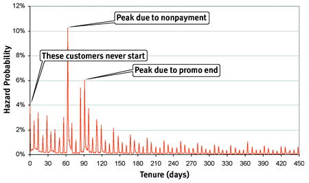
A picture paints a thousand words. Figure 1 charts hazard probabilities for customers in a typical subscription business. The horizontal axis is the tenure of customers measured in days; the vertical axis is the probability that customers stop at a particular tenure point.

FIGURE 1 Hazard probabilities for customers in a typical subscription business.

The hazard chart in Figure 1 is an X-ray into the customer life cycle because it highlights different important events. The first hazard probability at time zero is about 4 percent; this bump is due to customers not starting and is often caused by poor customer information being gathered at the point of sale or perhaps by buyer's remorse. At around 60 days, there's a very strong peak in the hazard probability. This peak corresponds to those customers who start but never pay. The company moves customers through various dunning levels to inspire payment. However, at some point, the company must force churn because of nonpayment. Changes in this policy, such as a reduction in the period of time for cutting off nonpaying customers, would be apparent in the hazard probabilities.

At around 90 days, we see another significant spike in the hazards. This spike actually has nothing to do with nonpayment. It's due to the end of the initial promotion. Customers who signed up for this service because the initial offer was cheap often stop when they have to start paying full price. Happily, the customers who stop at this point have at least been paying their bills.

After these two initial peaks, the hazard probability gradually declines, but with a jagged characteristic. The jaggedness is actually due to the one-month billing cycle that most customers are on. Customers are more likely to stop at the end of a billing cycle. One reason is that when customers call in to stop, the stop date is set to the end of the billing cycle unless the customer requests a specific date.

The gradual decline in hazards is also interesting. In fact, it says something quite important about customer loyalty: The longer customers stay with the company, the less likely they are to leave. The long-term decline in hazards is as good a measure of loyalty that I know.

From Hazards to Survival

If hazard curves provide an X-ray into the customer life cycle, survival curves provide a more holistic picture. The survival at time t is simply the likelihood that a customer will survive to that point in time. This is calculated directly from the hazards, by taking the cumulative probability that someone doesn't stop before time t — that is, by multiplying one minus the hazards together for all values less than t.

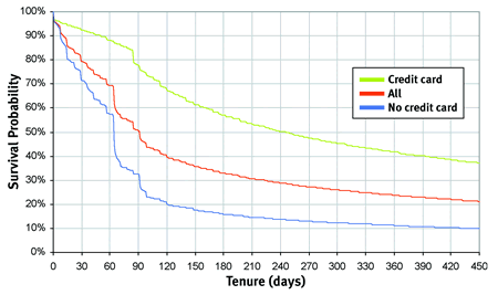
Figure 2 shows three examples of survival curves. Notice that all three curves start at 100 percent and gradually decline, with the survival value always between zero and 100 percent. The middle curve corresponds to the hazards in the earlier chart. Remember that the hazards had a spike around two and a half months. On the survival curve, this spike is instead a steep decline, indicating that customers don't survive beyond this point. So, this curve is saying that about 55 percent of customers survive beyond the nonpayment period. Once this period has passed, though, the survival curve flattens out, corresponding to the decline in hazards. Figure 2 shows that the smaller the hazards, the flatter the survival curve; and the larger the hazards, the steeper the survival.

FIGURE 2 Three examples of survival curves.

The other two curves in the chart help explain why. The top curve is for customers who started as credit-card paying customers. These customers provide a credit card, which is charged automatically every month. As the survival curve shows, there's no dip at two and a half months. These are paying customers. Almost 90 percent of them are still active after the initial nonpayment period, and their survival remains relatively high. These are good customers who don't disappear quickly.

The lower curve is for customers who are billed and pay by check rather than automatically by credit card. The survival curve for these pay-by-mail customers shows a much sharper drop. By looking at the stop reasons for these customers, it's apparent that this particular drop is due to nonpayment.

The middle curve is the "average" of the credit card and pay-by-mail customers. What's interesting is that the non-credit card customers are driving the entire drop for initial nonpayment. The survival curve graphically shows this common business wisdom.

Quantifying Survival

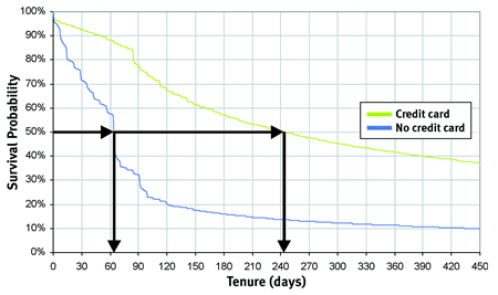
Survival does more than show the difference between groups of customers. It makes it possible to quantify the difference between groups. The chart in Figure 3 illustrates one common measure, the customer half-life (or median customer lifetime). This tenure is where exactly half of the original customers would still be expected to be active. The calculation is quite easy. The vertical axis has the survival values. Follow the 50 percent line over until it hits the survival curve. This is the tenure where half the customers "survive."

FIGURE 3 The customer half-life provides a good way to compare different groups of customers.

Figure 3 shows the median tenure by payment type for the groups shown earlier. For credit card payers, the median is more than 240 days; for others, it's barely a quarter of that. The customer half-life provides a good way to compare different groups of customers.

One drawback to the customer half-life is that the survival curve may not cross 50 percent. This means that the customer half-life isn't known, because the time window isn't large enough. Extrapolating survival beyond the time window is dangerous because what happens to customers isn't known. Customers may stay around for another 100 years, or they might all stop the next day.

The customer half-life is a good comparison for different groups of customers. However, this value only tells us about one customer — the customer whose tenure is exactly in the middle. A more useful number is the average customer lifetime, which can be dropped directly into customer value calculations. If a subscription is worth $500 per year in revenue and the average customer lifetime is 2.5 years, then the customer is worth $1,250 (assuming no discounting of future revenue).

Calculating the average tenure is conceptually quite easy. It turns out that the average tenure for a given time period is the area under the survival curve. For instance, the average tenure in the first year after acquisition for customers who stop half way through the year is half a year. On the other hand, customers who survive longer than one year only get one year because the calculation is only looking at the first year tenure. The average for all customers is the area under the survival curve, up to 365 days.

Competing Risks

Another critical idea in survival analysis is that of competing risks. When studying the survival rates for cancer victims, what happens when someone enrolled in the study dies in a car accident? Or moves to a foreign country? In medical terminology, these patients are "lost to follow-up." The same thing can happen with customers.

A clear example of competing risks is the distinction between voluntary and involuntary churn. Some customers are forced to leave (typically due to non-payment) whereas others leave voluntarily. When looking at churn, sometimes models are built leaving out one or the other group of customers. This, however, results in a biased model, which is an important issue when developing payment risk models separate from voluntary churn models.

With competing risks, the approach to the problem is a bit different. Customers who voluntarily stopped at a particular tenure — say one year — didn't stop either voluntarily or involuntarily before then. This is useful information for understanding both types of churn. Calculating competing risks follows the same pattern described earlier, with one difference. For each tenure period, a separate probability exists for each risk; once a customer has succumbed to one risk (say voluntary churn) the customer is no longer included in the population at risk for any of the risk groups. Technically, the customer is censored from other risks.

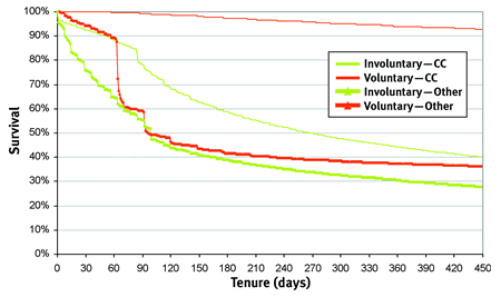
Figure 4 shows competing risks for voluntary and involuntary churn for the credit card paying and non-credit card customers shown earlier. The top line shows clearly that credit card paying customers are at minimal risk for involuntary churn.

FIGURE 4 Competing risks for voluntary and involuntary churn.

Although the canonical example is voluntary versus involuntary churn, estimating competing risks is useful in other situations. For instance, some customers may churn because they migrate to a higher value product. A wireless customer upgrading to more advanced technology may count as churn on the old technology. A cable subscriber who switches to digital cable may count as churn on her previous account. These examples suggest including migration as a competing risk for understanding these customers.

Addressing Other Problems

Survival data mining is not only applicable to churn, but is also applicable to almost any time-to-event problem. Survival data mining answers the question of when the next event will occur, rather than whether the event will occur in a certain period. Many opportunities exist for applying this technique.

When will a lapsed customer return? This is quite similar to the churn problem, but with one difference. Now the "start" is when a customer stops because it is the start of the lapsed period. The "end" is when (if ever) a customer restarts because it is the end of the lapsed period. You can apply the basic ideas of survival data mining to this situation. One challenge here is matching new customers to lapsed customers. Sometimes this information is readily available (for example, when the customer retains an identification number, such as a customer number or a telephone number). In other cases, householding algorithms can infer this information using names and addresses.

When will a customer next make a purchase? Understanding customers over time is a typical retailing challenge. Part of the question is when to start worrying that a customer hasn't returned. The survival data mining approach is to answer the question of how much time until the next purchase.

How long will an upgrade last? When customers upgrade to a new service, sometimes they eventually downgrade again. This is a competing risks problem, because customers might downgrade or stop during the period when they have upgraded. Upgrade survival curves are very useful for quantifying the value of the upgrade effort.

As the examples in this article show, survival data mining is a valuable tool for understanding customers and quantifying customer relationships. The basic techniques, borrowed from the statistics of medical studies, are moving far beyond the small studies that were their first applications. Survival data mining techniques are now proving their worth in the larger business world.

Calculating Hazards in a Database

Let's take a closer look at how survival data mining works with a database-in this case, running with Oracle's DBMS. Assume that a database contains one row for each customer with the following information:

How is this data used to calculate hazards? Fortunately, SQL does most of the calculations; Oracle extensions make the full calculation possible. The first thing is to calculate the tenure and the stop flag:

SELECT ((case when stop_date is NULL then < today >
else stop_date end) - start_date) as tenure,
(case when stop_date is NULL then 0
else 1 end) as is_stopped
FROM customers

The next step is to aggregate these fields by tenure. This gives the number of customers with exactly each tenure and the number that stopped with the tenure (some customers with the tenure will still be active):

SELECT ((case when stop_date is NULL then < today >
else stop_date end) - start_date) as tenure,
count(*) as pop_at_t,
sum(case when stop_date is NULL then 0
else 1 end) as num_stopped
FROM customers
GROUP BY ((case when stop_date is NULL then < today >
else stop_date end) - start_date)

At this point, you could continue the calculation in a spreadsheet. However, Oracle's analytic functions make it possible to calculate the total population at risk, and thus the hazard. The total population is the sum of pop_at_t for all tenures greater than or equal to t. The hazard is num_stopped divided by this total. The following query does this calculation (assuming the previous query is the subquery):

SELECT tenure,
sum(pop_at_t) over
(order by tenure desc range unbounded preceding),
num_stopped /
(sum(pop_at_t) over
(order by tenure desc range unbounded preceding))
FROM < subquery >
GROUP BY tenure
ORDER BY tenure

This example shows how hazards can be calculated directly from the database. This technique, however, does require SQL extensions, such as those that support Oracle's analytic functions.

Gordon S. Linoff [[email protected]] is founder and principal of Data Miners and is an expert in data mining and data warehousing. He is coauthor of Mining the Web, Data Mining Techniques, and Mastering Data Mining, all published by John Wiley & Sons. Prior to Data Miners, Linoff worked with Thinking Machines Corp.